
Our October 13 blog post “Rebalancing the Colorado River Basin: How Much Must Be Cut and What Will It Cost?” provided an overview of the water shortage in the Colorado River Basin (CRB) and summary of fallowing payments in existing programs. In this new post, we discuss the magnitude of potential cuts and a couple of alternative ways the cuts could be implemented based on current agreements and water right priority. Then we develop a simple economic analysis to illustrate the effects of cuts, including a least-cost scenario that would minimize economic losses to the Lower Basin.
Several announcements have been made since our initial post. Notably, the Bureau of Reclamation (Reclamation) announced an open solicitation for the newly formed Lower Colorado River Basin System Conservation and Efficiency Program (LCCP). The LCCP offered compensation ranging from $330 to $400 per AF for a one- to three-year agreement for water conserved and left in Lake Mead. The LCCP also allowed for other proposals with higher prices if supported by economic justification. Our earlier blog post noted some economic justifications for higher prices, namely: high prices for forage and other crops under current market conditions, the scale of conservation needed from fallowing, and drought conditions across the Western U.S. Reclamation accepted proposals for its LCCP through November 21, so additional news should be available soon.
Other recent developments include:
- Coachella Valley Water District executed an agreement with Reclamation to reduce imported water for its recharge facilities for $260 per acre-foot of consumptive use, for approximately 9,000 acre-feet.
- California users continue to pursue options for voluntary conservation of up to 400,000 acre-feet. However, specifics of any deal(s) have not been made public.
- Southern Nevada Water Authority released a proposal for revising the Lower Colorado River shortage guidelines, including a proposal to allocate evaporation losses according to each user’s diversion location and proportionate consumptive use.
- California has been slammed by a relentless stream of storms dropping rain and snow across the state. These storms have moved east but dropped most precipitation in Upper Basin states (mostly Utah). Stay tuned for a future blog post from us on the economics of infrastructure to capture water from large weather events.
Hypothetical Scenarios to Achieve a Reduction of 2 Million Acre-Feet
Last summer Reclamation announced a target for reducing consumptive use in the CRB by 2 to 4 million acre-feet (MAF). The size of the cuts falls outside anything encompassed in existing agreements. Voluntary agreements to cut water use so far appear to fall well short of the 2 MAF minimum target.
We developed three scenarios for how that 2 MAF cut could be achieved and assessed economic effects. One scenario used a trading analysis to explore lowering the total costs of achieving 2 MAF of cuts in the three Lower Basin states. The scenarios are:
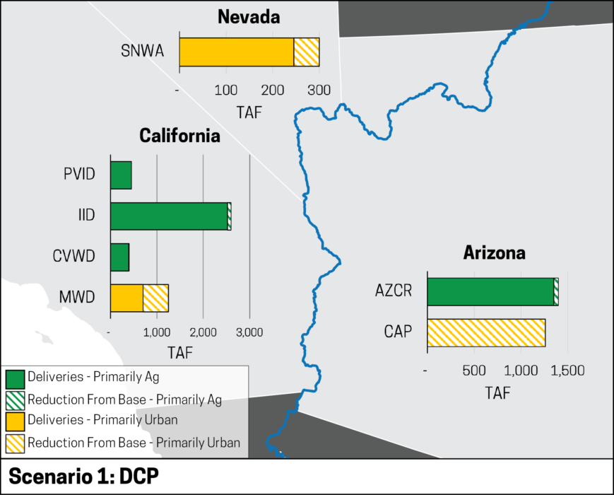
- DCP Scenario. The 2 MAF cut would be distributed among the Lower Basin states by proportionally increasing the DCP Tier 3 cuts (totaling approximately 1.1 MAF) to 2 MAF. Within California and Arizona, the cuts are imposed according to established priorities.
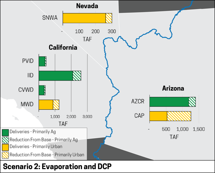
- Evaporation and DCP Scenario. This scenario starts by allocating evaporation losses among users based on SNWA’s proposal. Then remaining cuts needed to achieve 2 MAF are allocated according to DCP and within-state priority as in Scenario 1.
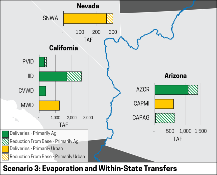
- Evaporation and Within-State Trading. This scenario builds on the Scenario 2 assumptions, including the evaporation losses. An economic model then allows for water trading within California and within Arizona to reduce the total cost of achieving the cuts.
We simply compare these three scenarios but make no claim about the legal validity or political palatability of any. Other allocations are certainly possible, and we note that the DCP was not constructed with these magnitudes of cuts in mind. For scenario 3, we emphasize that this is a preliminary look at where the cuts could occur, and the range of prices needed to stimulate voluntary participation.
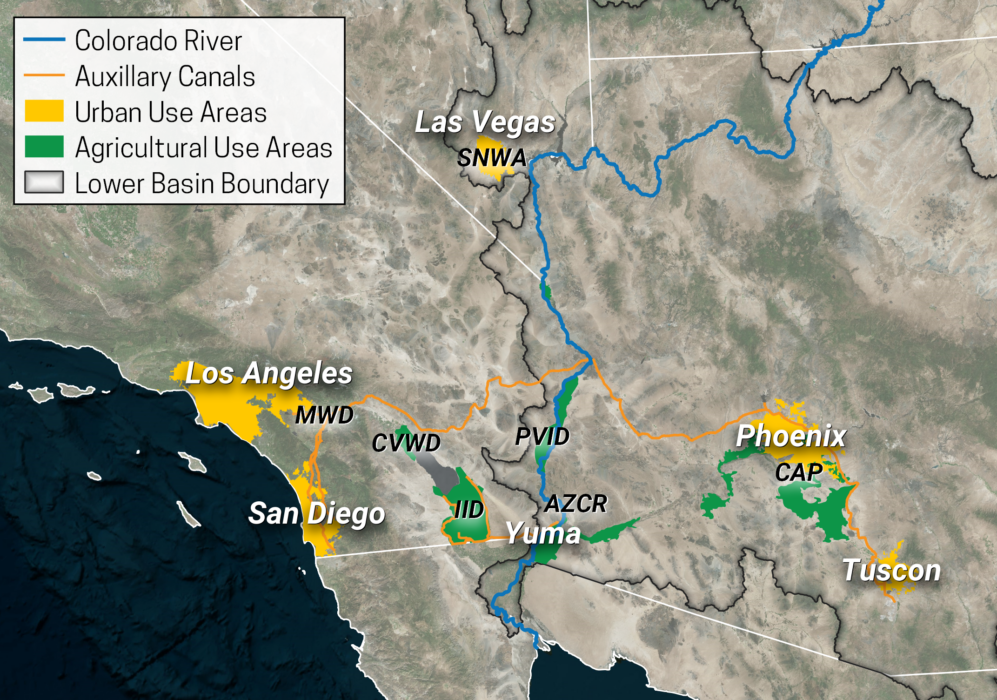
We defined eight aggregate regions that represent the major CR water users and water right priorities within each state (see Figure 1). Five of the water use regions provide mostly agricultural supply. These are: Coachella Valley Water District (CVWD), Imperial Irrigation District (IID), and Palo Verde Irrigation District (PVID) in California, agricultural water users on the Central Arizona Project (which we call CAP-Ag), and Arizona water users diverting from the mainstem of the Colorado River (which we call AZ-CR) in Arizona. Three of the water use regions are primarily municipal and industrial (M&I) users. These are: Metropolitan Water District of Southern California (MWD) in California, municipal and industrial uses on the Central Arizona Project including Phoenix and Tucson, (which we call CAP-M&I) in Arizona, and Southern Nevada Water Authority (which we call SNWA) in Nevada. For presenting results, agricultural and M&I uses on the CAP are grouped together in Scenarios 1 and 2 (which we call CAP). We do not include tribal water delivered by CAP in this curtailment analysis.
In each scenario we estimated the amount of Colorado River water cut from each state and region. Many regions have a portfolio of Colorado and non-Colorado River water supplies, including existing exchange agreements, which we analyzed to determine the total water supply in each region. We calibrated an economic model of the demand for water in the Lower Basin regions and applied that to evaluate the impact of each scenario. We describe outputs in terms of net reductions in water supply and the cost of that reduction (measured as losses in economic well-being). We used regional demand elasticities representative for the different uses of water, along with recent estimates of regional quantities and marginal use values, to calibrate water demand functions for each region. It is important to note that the water values are not the water rates charged by the agencies to their customers but reflect the marginal cost of alternative supplies or shortages. Some numbers we use are representative values or assumptions for this analysis, such as the demand elasticities and the split between CAP agriculture and M&I use.
Results
The Scenario 1 cuts fall unevenly across regions based on the DCP Tier 3 shares and different water rights priorities within states (Figure 2a). This results in disproportionately higher cuts to CAP and M&I in California and Nevada. MWD’s CR allocation would go to zero, though it would continue to receive CR water though existing agreements with agricultural water districts. In Arizona, users on the Central Arizona Project experience higher cuts compared to the agricultural users on the Colorado River, which have higher priority. Our example model estimates that Scenario 1 cuts would impose costs that fall primarily on urban water users.
The allocation of evaporation in Scenario 2 results in a different distribution of cuts (Figure 2b). In Scenario 1, IID, which has more senior rights, is cut little. In contrast, evaporation losses in Scenario 2 fall more heavily on the large users lower in the basin, especially IID. Our example model estimates that Scenario 2 cuts would impose less total cost than Scenario 1 because cuts are distributed across both agriculture and urban water users.
Scenarios 1 and 2 allocate 2 MAF in cuts based on rules that do not consider economic costs of cuts. The value of water varies by use and region, with M&I users facing substantially higher costs than agricultural users. This suggests that there is potential to lower the cost of cuts through compensated, voluntary trading. We developed an example analysis to illustrate within-state trading to reduce the total cost of implementing 2 MAF of cuts in the Lower Basin; this is Scenario 3. In Scenario 3, we evaluate potential transfers between agricultural and M&I uses within each of Arizona’s and California’s CR water users. The trades begin from the Scenario 2 allocation rules. Figure 2c illustrates the resulting distribution of water delivery. As expected, based on the difference between agricultural and M&I water values, this scenario reduces costs by shifting water cuts away from the urban uses in California and Arizona, allowing the sale of water to these regions, largely from IID and CAP-AG but also from the AZ-CR and PVID regions. In this analysis we have excluded SNWA from any transfers, but that can be included in another scenario. Our example estimated that trading would reduce the total economic cost of cuts by about 55 percent relative to Scenario 2. This does not include any transaction costs for negotiating and executing deals, so this should be viewed as an optimistic estimate of the total cost savings from Scenario 3.
In this initial analysis, after-trading unit values of water remain higher for M&I buyers than for agricultural sellers, reflecting conveyance and institutional constraints that prevent a market-clearing equilibrium to occur.
The difference in unit values between buyer and seller leaves significant room for negotiating a mutually beneficial deal, in which agricultural water users could be well-compensated for water cuts. To date, payments for water trades in the Lower Basin appear to reflect the compensation needed to fallow agricultural field and forage crops (the obvious exception being San Diego CWA’s payments to IID for efficiency conservation), rather than the M&I buyers’ higher willingness to pay for water. Given the scale of cuts considered here, we expect higher prices that fall somewhere between sellers’ and buyers’ water values.
Our next blog discusses other economic impacts and considerations for how to move forward.
If you’re interested to talk more about the Colorado River Basin shortages and related economic impacts, reach out to Steve Hatchett.